Thursday 20 December 2012

Principles of Economics - Perfect Competition

Perfect Competition is a market structure that follows these assumptions:

  • Firms are price takers - each firm has no impact on the price in the market, they take the price the market forces set.
  • Freedom of entry into the market - there are low barriers to entry so anyone could potentially set up in this market.
  • Firms produce identical products - the taxi market for example, each taxi firm offers an identical product.
  • Producers and consumers have perfect knowledge - both producers and consumers know everything there is to be known about the market.

However, few, if any, industries are actually perfectly competitive.

In the short run, the number of firms is fixed. In the long run, if supernormal profits are being made then new firms will enter the industry. If losses are being made, firms will leave the industry. 

Short run equilibrium of the firm:


This is what the market looks like in the short run in perfect competition. The price is Pe, and is set by the demand and supply forces. It is horizontal because firms are price takers. Due to price being constant, the red dotted line is also the average revenue, the marginal revenue and the demand for the firm as they're all the same. Qe is the amount produced by the firm because this is the amount at which profits are maximised (MC = MR). There is slight profit being made because the average revenue is higher than the average cost at the production point.

This is where the long run can be introduced. In the long run, firms see these profits being made and enter the industry. These means the industry supply increases, shifting the supply curve to the right on the left hand diagram above. Price falls, which means each firms demand falls until the point it is equal to the average cost. At this point, firms break even and make no profit. Firms will stop entering the industry now.

As far as the public interest goes with perfect competition, it has its benefits and drawbacks. The benefits are as follows:

  • Firms produce at the least cost output.
  • Firms that are inefficient will be forced out.
  • Prices are minimised.
  • Consumers determine what and how much is produced.

The drawbacks are:
  • There us very little incentive to invest in new technology.
  • Goods are all the same, lack of variety for consumers.

That ties up this post about perfect competition. Thank you for reading, keep checking back and sharing. Have a good day!

Sam.


Saturday 1 December 2012

Common Agricultural Policy Part 3 - Buffer Stocks

A tool at the EU's disposal within the CAP is buffer stocks. They can use these to either stabilise the prices of farm produce or to stabilise farmers income.

First case we'll analyse is the case of buffer stocks being used to stabilise prices of farm produce.


We have a market for a crop here, Q1 and P1 being the equilibrium quantity and price respectively. Lets assume one year there is a good harvest, supply increases to S1. We notice that this would create a fall in price, however as the policy is aiming to stabilise prices this isn't what we want. So, in order for this supply increase to come with stable prices, the governments need to buy up the difference between Q1 and Q2 and put them into buffer stocks. This means, the quantity available to the public is the original level of Q1, and therefore price won't change. 

Alternatively, if there is a bad harvest and supply falls to S2, a price rise would occur. The governments would have to intervene here and sell the difference between Q1 and Q3 to the market, releasing them from buffer stocks so the quantity available is the same and therefore the price remains stable. 

The areas on the diagram represent a few different things. Area a is an income that the farmers are guaranteed, even in the worst times. Area a + b is the normal income for a farmer, assuming that the harvest is a normal one. Area c is extra income the farmer would earn given a good harvest. Notice this policy of stabilising the farming prices has created more fluctuation in the farmers incomes, something the CAP aims to eradicate. Controversial.

Now, onto how buffer stocks can be used to stabilise a farms income. This involves using the elasticity formula. If elasticity of the good equals to 1, then the percentage increase in quantity is the same as the percentage fall in price. Therefore, if these are the same then the income of the farmer will remain constant. 


This diagram shows the principle of stabilising a farmers income using buffer stocks. We have an initial equilibrium of P1 and Q1, and supply increases because of a good harvest. This essentially means that a new equilibrium will be formed at P2 and Q2. However, at this point the farmers income has changed because demand doesn't have unitary elasticity. Therefore, the government needs to intervene. Using the curve above, we can see where the price and quantity should be for farmers income to remain stable: P2' and Q2'. So, what the government needs to do is buy up the difference between Q2 and Q2' and put them into buffer stocks. This means that the quantity now available will mean that price is at P2' and therefore farmers income will be stable. We can see this visually, the farmer has lost area c in terms of income due to the price fall,but gained area a + b due to the increase in quantity. These areas should be identical and therefore the farmers income has remained constant. 

This concept also works the other way if supply were to fall. Just in this case the governments would be releasing from the buffer stocks in order to regulate the price and quantity so that the farmers income remains stable. 

Buffer stocks is one method the government has to try and stop price fluctuations or income fluctuations, however it cannot be used to control both at the same time. Next up will be the use of subsidies for the same reasons. 

Sam.

Statistics - Sampling Methods and Estimation

In statistics we have to use samples because it's normally near on impossible to get data for the entire population. As long as the sampling is done well, the results will usually be good enough. Logic would tell you that the larger the sample, the better.. and this is true. There are two concepts we need to understand here, those are random sampling and sampling distribution.

  • Random sampling - The goal of this is representativeness, we aim to get an equal probability of selection to every member of the population. There are a few methods:
    • Simple random sampling - A sample so that every item or person in a population has the same chance of being included.
    • Systematic random sampling - Items or individuals are arranged in some sort of order. A random starting point is selected and then every nth member is selected. Alphabetic order for example. 
    • Stratified random sampling - A population is divided into sub groups (strata) and a sample is selected from each strata.
    • Cluster sampling - A population is divided up into primary units and then samples are selected from the primary units.
    • Non-probability sampling - Inclusion in the sample is based on the judgement of the person selecting the sample. (Eeek!)

  • Sampling Distribution - This is the theoretical distribution of a statistic for all possible samples of a certain sample size, N. It's a device to link the samples characteristics to the population.
    • If repeated sample sizes of size N are drawn from a normal population with a mean of mew and a standard deviation, σ, then the sampling distribution of sample means will be normal with a mean of mew and a standard deviation of σ / SqrRoot(N).
    • The 'Central Limit Theorem' states that if repeated samples of size N are drawn from a population, as N becomes large the sampling distribution or sample means will approach normality.
    • Or, in easier terms: Large samples are more reliable!

The more basic method of estimation is confidence intervals. From a sample we don't know the population mean, but we would like to estimate this with maximum efficiency. To do this we use a range, and say how certain we are that this range includes the population mean. We give a confidence interval in the form of a percentage, for example we could say that at a 99% confidence interval, between 33% and 39% of adults will vote for Labour in the next election (Made up!). A bigger confidence interval is more likely to contain the true population mean.

The next post will go further into the concept of confidence intervals and we will introduce such things as error margins. Stay tuned, thanks guys!

Sam. 

Friday 30 November 2012

Common Agricultural Policy Part 2 - Declining Farm Incomes

The next thing the CAP aims to eradicate is declining farm incomes. These are mainly caused by two things: low income elasticity of demand and/or increases in supply. As usual, we'll display this diagrammatically. Lets suppose we have a fairly inelastic demand curve and at the same time farm efficiency has improved, we can expect the market to now look as follows:


We can see that prices have fallen from P1 to P2 and quantity has risen from Q1 to Q2. However, we can also see that this has caused a fall in income of area a and an additional income of area b for the farmers. Area a is clearly larger than area b, meaning the farmers income as a whole has fallen. The way for farmers to gain is for demand to shift out by a larger amount, as even a small shift in demand would leave farm incomes still falling. 

What the farmers need is a more elastic demand curve for any increases in supply efficiency to actually increase farmers income. However, demand for grown crops is generally more inelastic because it's a necessity and therefore a change in price really doesn't affect demand all that much. This is why the government needs to intervene with the CAP because else there would be no incentive for farmers to make their production mechanisms more efficient as they'd effectively be losing money due to it.

Now we have covered both reasons as to why the CAP is necessary; fluctuating crop prices and declining farm incomes. We will next cover how the EU uses it's policies to correct these issues. Stay tuned!

Sam.


Statistics - The Normal Probability Distribution

This post will bring in an application of standard deviation. It can help give us units to measure distances between points in a data set as well as to measure the distance from the mean.

Chebyshev had a theorem. He said that for any set of observations, the minimum proportion of values that lie withing k standard deviations of the mean is 1- (1/k^2), as long as k is greater than 1. If k is 3, 89% of the observations lie withing the region and if k is 4, 94% of observations lie within the region.

For a normal probability distribution we need to use a normal curve, or a bell curve. It has a single peak in the centre of the distribution. This centre point is where the mean equals the median equals the mode. We can now introduce a new concept of z-values. A z-value is the distance between a selected value (Xi) and the population mean, divided by the population standard deviation. Another note on the normal curve is that is has a Kurtosis of 0. A higher Kurtosis means it's peak is higher and more pointy, a lower Kurtosis means it's a flatter shape.

Back to the z scores. They link together the theoretical normal distribution to the observed observations. It tells us how many standard deviations away from the mean an observation lies. So, we need to calculate the z-score. When calculating the z score it is essentially converting your data into a distribution with a mean of 0 and a normal curve shape. The formula is as follows:


Once the score has been calculated, you refer to a z score table. On this table, the first decimal goes down the side and the second decimal goes along the top. So, if using the formula above you were given a z score of 1.24, then you'd look for 1.2 down the side and 0.04 along the top. The score at which these match is your z score. That score is 0.3925. What to do with that score becomes more understandable with an example and some context. 

At a party, lemonade is distributed among the party-goers with a mean of 20cl and a standard deviation of 5cl. What is the likelihood that a person selected at random will get between 17cl and 23cl of lemonade? Right, so we plug in the values to start. z will equal (17 - 20) / 5 = -0.6. It will also equal (23-20) / 5 = 0.6. Now, from here we look for 0.6 down the side of the z score table and 0.00 along the top. We will be given a value of 0.2257. This score caters for one of the results, but as they are both the same size we can double it and get 0.4514. And that's the answer. 45.14% of people get between 17 and 23cl of lemonade, so the likelihood of any given person getting between that amount is 45.14%.

Another use for z scores isn't just finding the amount included, it can be used to find excluded regions too. That may sound quite complex, but I'll show you a picture to visualise it.


We need some context once again to work this out. Let's say that a teacher has said to achieve an A* on a test, students must get in the top 10% of the scores. The mean score for the test was 75 and there was a standard deviation of 5. We can now work out what score is needed to get a A*. The whole region to the right of the mean makes up 50%, we know we want to exclude 10%, so we need to find a z-score that marks 40% - 0.4. On the z-score table 0.4 doesn't appear (remember this time we know the size of the region, so we are looking at the values in the table and looking for a corresponding z score), 0.3997 is the closest so we'll go with that. That gives a z-score if 1.28. Now we need to refer back to the z score formula. We know z, we know s and we know the mean... we are trying to work out Xi. So, we plug in the numbers we have an rearrange to find Xi. 1.28 = (Xi - 75) / 5. Xi - 75 = 6.4. Xi = 81.4. There we have it, the answer. To make it more realistic this score could be rounded to 81 or 82, but one of these scores is needed to achieve the top 10% of the class and therefore get an A*. Simples!

That's it from me, z-scores are a fairly complex topic so feel free to ask any questions if i haven't been entirely clear in the explanation. Good luck!

Sam.


Tuesday 27 November 2012

Common Agricultural Policy Part 1 - Price Fluctuations

The Common Agricultural Policy is a massive deal in Europe and the European Union. It's a very expensive policy that started out back in 1962 as a simple price support policy. It has two key objectives: to stabilise prices and to provide income support for social reasons. If you look at the distribution of farms across Europe, it is clear to see why this is needed. The biggest 7% of farmers own roughly half the land, whilst the smallest 50% of farmers own only 7% of land. This is a massive inequality and could lead to monopoly powers, outlandish prices and other such problems if it went unregulated.

We'll first look at a few of the characteristics of the agricultural industry. There are many producers, all are price takes. There are also many consumers, all of which are also price takers. There is generally freedom of entry and exit into the industry. It's about as close to perfect competition as you could get in a realistic scenario. Governments need to intervene for many reasons:
  • To reduce price fluctuations.
  • Raise farm incomes.
  • Protect rural communities.
  • To encourage greater self-sufficiency.

Firstly, I'm going to focus on the price fluctuations. In the short term they are caused by instability and the fluctuations in the harvest (good or bad!). Let's assume that the demand for a crop were to rise one year, which would cause a shift to the right of the demand curve. Supply in the short term obviously cannot react to this because supply is fixed each year depending on what is planted. This demand rise will cause a rise from price P1 to P2. This is all shown on the diagram below.


The farmers observe this rise in price and then next year they increase their supply to the market. At P2 the farmers decide that Q2 is the correct quantity to supply to the market. However, at this amount supplied, demand is outstripped and therefore price must fall to P3. The year after, at price P3 a different amount is supplied by the farmers, but at this supply more is demanded and therefore price rises again. This will continue, as shown on the diagram below we can see that the market is slowly spiralling towards a point of equilibrium at which both consumers and producers would be happy. 


We call this concept a stable cobweb. This price fluctuations and changes are supply are making the market more and more stable as over time the fluctuations get smaller until equilibrium is finally met. In this case, the government wouldn't need to intervene in the agricultural industry. However, there is the opposite case. An unstable cobweb could appear. The case of this occurs when the supply of the crop is very elastic. Diagramatically, the supply curve will be much flatter. The same instance as above will occur, demand increases causing a price rise as supply is fixed. In the second term supply is increased due to this new price, but there is oversupply and price has to fall... and so on and so forth. Except, when the supply curve is elastic this doesn't spiral towards equilibrium, it spirals away from it as can be seen in the diagram below.


This shows one of the cases in which the government would need to intervene in the agricultural industry, hence the Common Agricultural Policy. The price fluctuations in this unstable cobweb would keep getting worse and worse if left to market forces. 

Next we'll move on too supply side shocks. This is when supply is affected, either for good or for bad, and therefore the supply of the crop isn't as expected. Once again, diagrams are an easier way of showing this. The first case will be a bad harvest, where supply of the crop is less than what was expected. The diagram below shows this. Supply of the crop has fallen from the expected level of Qe to the actual level of Qa. The area labelled 'b' is income that the farmer has lost, the area labelled 'c' is income gained from this supply side shock. The expected income for the farmer was area 'ab', but the actual income of the farmer is now area 'ac'. If area c is greater than area b then the farmer has gained, otherwise the farmer has lost out due to the bad harvest. Generally, the more inelastic demand is, the greater are 'c' is and therefore the more likely the farmer will benefit. 


I'll quickly go through the other supply side shock as well. As you can guess, this is when there is a better harvest than expected. This causes a shift to the right of actual supply from Qe to Qa. A fall in price is seen from Pe to Pa and once again the farmers income may be affected. Area 'c' is the income gain, area 'b' is the income loss and area 'a' is the income that has stayed constant. If area 'b' is bigger than area 'c' then the farmer has lost out. 


What we have achieved in this blog post is the causes of the fluctuations in prices of harvested goods. This is one of the things the Common Agricultural Policy aims to stop, as stable prices is an aim. In the next post we'll look at what is causing the decline of farmers income and then we'll move on to look at how the government intervenes in this policy to correct these issues.

Stay tuned guys, enjoy!

Sam.


Statistics - Measures of Dispersion

The first measure of dispersion of data we'll mention is the range. The range is the difference between the highest value and the lowest value in a set of data. Only these two values are used in the calculation and it is very easy to compute. It has a slight issue, however, that extreme values do influence the result. 

A step on from this range is the interquartile range. This is the difference between the first quartile and the third quartile - giving us the middle 50% of observations. To work out the first quartile, we take N (number of observations) and divide it by 4. This will give us the number of the observation at which the first quartile point is. To work out the third quartile we take N and divide it by 4 and then multiply the result by 3. This gives us the number of the observation at which the third quartlile mark is. From there, we just subtract the value of the first quartile figure away from the third quartile figure. 

The quartiles are then displayed on a box plot diagram. A box plot will look generally as follows:


Mean deviation is another measure of dispersion. This measures the mean of the absolute values of the deviations from the mean. Similar to standard deviation, but not quite. The formula is as follows:

  • Mean Deviation = (Σ|Xi - x̄|) / n
  • Xi = each observation
  •  = the sample mean.
  • n = number of observations.

We take the absolute values here for a very specific reason. It stops the negative and positive values from cancelling each other out, which would give us a mean deviation of close to 0 - very unhelpful! Dispersion is very important, key statistical methods such as regression rely heavily on measures of dispersion. 

The population variance and sample variance are two more concepts I'm going to introduce now. The population variance measures the arithmetic mean of the squared deviations from the population mean. The sample variance essentially does the same, but for a sample. The formula for both are as follows:

  • Population variance = (Σ|X - μ|)^2 / N
  • Sample variance = (Σ|Xi - |)^2 / (n - 1)

These variances can be easily turned into the standard deviations, a very important concept for statisticians. To do this, we just square root the result. We denote the standard deviation of a population and a sample differently. A population is given with this symbol: σ and a sample is given with the letter s. The standard deviation principle will come in key in the next few posts when we begin to introduce confidence intervals, so learn it!

Thanks for reading, have a good day.
Sam.


Monday 26 November 2012

Statistics - Measures of Central Tendancy

By the end of this post I hope that you'll be able to characterise a data-set with one piece of information  and more importantly briefly describe complex data in simple terms. 

We'll start with the mean. The mean is computed by adding up all the values and dividing by the number of observations there are (N or n). Two symbols appear for means, these are x̄ (sample) and μ (population). If you take each score in a distribution and subtract the mean from it, and add all these differences the sum will always be 0. The mean does have some disadvantages, such as extreme scores pulling the mean one way or another. This issue doesn't occur with the median. To work out the population mean, or μ, all data in that population must be added up and divided by the population. For the sample mean, or x̄, all sample data must be added together and divided by the number of observations in the sample. 

A different type of mean to the arithmetic mean above is a weighted mean. This allows us to create accurate calculations even when all the information isn't known. It's fairly straight forward, like above. The formula for weighted means is as follows: x̄ = (w1X1 + w2X2 + ... + wnXn) / (w1 + w2 + ... + wn). 'w' here denotes the weight given to the value 'X', the higher the weight the more influence it has on the mean. If the weights are all 1 you essentially have the same formula for as the arithmetic mean in the previous paragraph. The problem with this is that sometimes the weights aren't known and outliers are very common in economics. 

Next, we move on to the median. This, as many already know, is the middle score when the observations are arranged in order. If there is an even number of scores, it's the mean of the middle two values. There is a unique median for each set of data. It isn't affected by extreme values and is therefore a very good measure of central tendency. 

The logical step now is to introduce the mode. The mode is the most frequently appearing value in a data-set. It is of limited use because it doesn't give any weighting to unique values. Other problems arise, such as some data having no mode and some having more than one. It really doesn't give a good measure of central tendency for a set of data. 

Skewness! A few graphs will crop up in this section. Skewness tells us in which direction the data swings, it is normally represented graphically. We start off with the bell curve. This is when the mode = median = mean, we have no skew and the data fits nicely into this 'bell' shape shown below. The distribution is symmetrical. 


A positively skewed distribution occurs when the mode < median < mean. The data is all bunched to the left of the mean and then it falters out. It looks like below.


Finally, the negatively skewed distribution. It's the stark opposite of above, the mean < median < mode. Here it is. 


You might have worked out by now, by skewness measures the lack of symmetry of the distribution. This lack of symmetry can be given a numerical value ranging from -3.00 to 3.00. A value of 0 indicates a symmetric distribution. It is worked out as follows: sk = 3(x̄ - Median) / s. 's' stands for standard deviation which will be coming up in the next blog post, so stick around for that. 

That's all for this post. I hope now you're able to describe your data set fairly easily, tell us the middle value, the average in which direction it's skewed and so on and so forth. It's a good tool to have, yet still very basic. We'll be stepping up another gear next post as range and deviations are introduced. Keep checking back, thank you guys!

Sam. 


Friday 23 November 2012

Statistics - Introduction

*Disclaimer: I have a statistics test coming up soon, so expect the next few blog posts to be all statistics related. I'll be getting back to normal economics after the 8th December. Statistics, however, is useful to people outside the discipline of economics as well as econometrics studies.*

I'll start at the very basics of statistics. This post will contain a few definitions and a few formulae, nothing too taxing as we're just setting the scene, so to speak. In statistics, we have two types of variable; a qualitative variable and a quantitative variable. The features of these are as follows:

  • Qualitative: Non numeric. For example: gender, religion.
  • Quantitative: Numeric. For example: bank balance, age. Can be either discrete of continuous.
    • Discrete - Can only have particular numbers. Example: Family members (Only whole numbers)
    • Continuous - Anything else. Example: Weight, height.

Data can define on different levels as well. We can have nominal, ordinal, ratio or interval data. Again, these all have different characteristics:

  • Nominal Data - Categorised data that cannot be arranged into an order. Eye colour, for example. This data can be either mutually exclusive and/or exhaustive. It's usually qualitative.
    • Mutually exclusive - Can only be included in one category. Only one eye colour for example.
    • Exhaustive - The data must appear in at least one category.
    • Gender is mutually exclusive and exhaustive.
  • Ordinal Data - Data that can be arranged into some sort of order. Individuals can be compared with one another here because of rankings, however the distances between each piece of data has no meaning.
  • Interval Data - Can tell differences between the distance of data, yet we still aren't able to say that 100 is twice 50.
  • Ratio Data - Has a 0 point, e.g number of family members. Now we can say that a family of 4 members is twice as big as a family of 2.

I'll now move on to looking at frequency distributions and how we can present these graphically. A frequency distribution is a grouping of data into mutually exclusive categories showing how many observations are in each class. A class is a subset of the whole range of the data, each class will be the same size and all the classes together will make up equal to or more than the range of data.

The class midpoint is the average of the upper and lower limits of the class. The class frequency is how many observations fall into that class. The class interval is the difference between the upper and lower limit of the class. 

There is a rule for how to divide your data into classes. It's named the 2 to the k rule. In this example we refer to 'N', this is the number of observations. The rule is you choose k so that 2 to the power of k > N. This value of k will be the number of classes. How to choose the size of these classes is fairly straight forward as well. Minus the upper score by the lower score and then divide this value by the k we just got from the last formula. A decimal value may well be given, in that case round UP to the nearest sensible number. The data can now be displayed clearly in a frequency distribution diagram/table.

Relative frequency distribution is essentially the same as above, except adding one more column in the table. This new column shows the percentage of observations in that class. Divide the amount of observations in that class by the total amount of observations and multiply by 100 to get the percentage. Simplez.

The data can be displayed graphically in many forms, none of them being 'wrong' per say. Histograms, frequency polygons and cumulative frequency distributions are examples of these graphical representations. These are all for examining data and trends in that data.

You may ask the question about line graphs here, when do we use these? In general, line graphs are used when time is involved. They can show the change over a period of time. Bar charts are for showing different categories that have no clear link, or to measure frequencies. Pie charts are simply for showing proportions. Scatter graphs show us co-variation of two variables, but NOT time. Any over diagram are subjective and not advised. 

Introduction to statistics complete! I hope that makes enough sense to you all, comment your problems if not and I'll get back to you ASAP. Thanks for reading, good luck!

Sam.  

Wednesday 14 November 2012

Principles of Economics: Profit Maximisation (Microeconomics)

Today's post will look at the profit maximisation for a firm. There really isn't that much too this, but I'll dedicate a post to it none the less. If you refer back to the post relating to a firm's revenue it will make what's about to be explained a lot easier. The main rule to remember here is that the profit maximising point for a firm is where the marginal revenue and marginal cost are equal. Why this point? Well, as long as marginal revenue is greater than marginal cost more profit can be made by increasing production. At the point where marginal revenue equals marginal cost, no more profit can be made and therefore this point will be the profit maximisation point.

Diagram time!

Profit maximisation is shown on this diagram here. We've set up a simple model of a firm's revenue and costs. Then, at the point MC = MR we have drawn a line up. This gives us two prices, P1 and P2. P1 is the actual market price for the good or service. P2 is the cost to produce that certain good. Therefore, using simple logic we can work out the actual price. P1 - P2 will give us the profit made on each good produced and then if we multiply this by the quantity we will have total supernormal profit. Or, visually it's the gold area on the diagram.

Notice I used the phrase supernormal profit. There are actually two levels of profit, normal profit and supernormal profit. Normal profit is the cost of staying in the industry; so this is essentially the minimum amount the firm needs to make in order to stop them leaving the industry. It will include such things as the pay for the entrepreneur. Supernormal profit is anything above this level, any additional income for the firm. A situation can also occur when the average cost curve is higher than the average revenue curve, if you picture this in your head and you'll see it'll result in a loss. In the short term some firms will not worry about this if they are using it as a technique to reduce competition or something similar. In this case nothing changes, the firm will still produce at the point MC = MR, however the only change is this time we'll call it the loss-mining position/quantity. 

Sorted! Profit maximsation and loss minimisation for you! Hope it helps, feedback and comments are of course always welcomed! Thank you guys, have a good evening.

Sam. 

Saturday 3 November 2012

The Transformation of Policy Between the Wars

Immediately after the First World War, the government's aim for policy was to get the economy back to the 'normality' experienced prior to 1914. This sort of thing included the government playing a limited role in the economy, more integration with the world economy and restoration of the gold standard, free trade and a balance budget.

Initially these three final points are achieved. The budget is eventually balanced, albeit a higher budget than previous years due to the increase social spending and maintenance of the national debt. During the 1920's the policy of free trade is also pretty much restored. Britain gets back on the gold standard in 1925 at the rate of £1 = $4.86. Germany and France both rejoin the gold standard at a similar time, along with most other leading economies. Why did we return to the gold standard you may ask? Well, firstly it helped achieve the restoration of pre-war 'normality'. Also, it aimed to try and stabilise the currency which would in turn help out trade. Another feature of the gold standard was to allow the monetary system to function on its own. What I mean by this, is that if the country runs a payments surplus then gold will flow into the country, interest rates will be decreased so wages and prices will fall. This will in turn cure the surplus. It also works the opposite way for a payments deficit. A final point is that the gold standard was a means of stopping politicians from meddling with the money supply!

However, pre 1914 the gold standard worked but after the war and during the 1920's it just didn't. There is a list of potential reasons for this:


  • Why the gold standard worked pre-1914:
    • It was developed gradually over time.
    • Capital and labour was freely moving.
    • The central bank could use interest rates to protect the currency, independent of the government. 
    • London was still a financial centre.

  • What changed in the 20's?
    • There was a rush to return to the gold standard.
    • More protectionism and less migration due to barriers.
    • Central banks were under pressure from politicians.
    • Paris and New York now competing against London as financial centres. 

Mr. Keynes pops up again in this debate. He pointed out that British prices had risen faster than the US', so starting at the same £1 = $4.86 rate would be an overvaluation of the pound. Although this shouldn't have matter because the gold standard should re-adjust prices, Keynes doubted it would work. He thought it would have bad domestic effects including interest rates needing to be kept at 4.5-4.5% and due to this borrowing would become expensive and investment would suffer.

The world slump is the next chronological step in the economic history of Britain. The recession of 1929 - 1931 started because of the Wall Street Crash in the US. This meant massive balance of payments problems. In 1931 came the European Banking Crisis and so in Autumn of that year Britain was forced off of the gold standard. This was first portrayed as a temporary change, but gradually the realisation came about that it was for good. Interest rates were cut to 2% to encourage borrowing and investment which would boost the economy again! Amazingly, there was a recovery. GDP rose as investment rose and Britain actually now compared well with other global economies. It would be easy to say all of this was because of the gold standard, but it isn't true as many other factors were also contributing to the recovery of the British economy. What the slump did cause, however, is the abandonment of free trade between 1931 and 1932. 

Keynes had the idea that investment from the government was something that was necessary for the economy. But, the treasury wasn't in agreement with this theory. They believed it would unsettle foreign investors and worsen the national debt. Keynes thought that there was no point in cutting wages because demand and consumption would suffer. What was needed was public investment which would boost the economy via the multiplier effect. The treasury argued it would be inflationary and any more borrowing would get out of control. The only time borrowing was allowed was in a one-off circumstance for rearmament!

Thanks for reading again guys, that'll be it for economic history for a while... I promise! Haha.

Sam. 

The Economy During Interwar Britain

We've seen how the economy functioned prior to war and during the First World War in the last few blog posts, now we'll move on to the economy between the two world wars. Instability is the major recurring theme in this period. We see two major recessions, one between 1920 and 1922 and another from 1929 to 1932. There's also a slight one between 1937 and 1938, but this wasn't as sever. If you look at this in context with the rest of the world, Britain's economy is actually relatively stable yet still under-performing comparatively to the other large economies. If we look at growth statistics we can see that in the latter half of the interwar era the economy was growing at a respectable 2.2%, however before this the economy actually shrunk and therefore the growth average for the whole interwar period (1913-1937) isn't at all impressive.

There were many weaknesses to the interwar economy, as you'd expect. Firstly, international trade was falling. We'd relied so heavily on it in the 1870-1914 period but now it was dwindling rapidly. In 1913, international trade and services was at 30% of GDP. In 1938 it was only 15%. The levels of trade did not exceed the 1913 levels until after the Second World War. One of the causes for this fall in trade is that world output grew faster than world trade. Essentially this meant that demand for Britain's goods would fall because the market was getting more competitive as supply was increasing. Here are some statistics to back that point up:

  • 1929 - There is 80% higher production of manufactured goods than in 1913.
  • Britain's market share for manufactured goods fell from 30% in 1913 to 22% in 1937.

An example of this downturn in trade can be seen in the cotton industry. In 1914, Britain was a net exporter of cotton, with 80% of what was produced being shipped abroad. Other markets around the world, such as India, began to become self-sufficient behind tariff walls and therefore didn't import as many. Other countries such as Japan began to produce cotton too at a lower cost because of the low-wages. Because of this British cotton exports halved over the period 1913 to 1936.

Another issue with the economy is the mass unemployment. In the good years it's still at 8%, in the worse years it could reach as high as 17%. However, the issue was mostly geographical, or regional. The north of England, Wales, Scotland and Northern Island were the worst affected. These ares tended to rely a lot on the older Victorian industries such as coal and cotton. In the South and the Midlands, new developing industries were adopted, such as cars and chemicals and therefore unemployment here was at a reasonable level. Old industries were failing and not enough new jobs were being created to keep the unemployment down. 

Some economists began to argue that the problem with the economy was an inflexible labour market after 1914. Why was this? Well, trade unions had gained a lot more power, there were generous unemployment benefits giving no incentive to find work and institutions could set their own minimum wage rates. This made wages pretty stuck and unable to change much to changes in prices. However, it isn't crystal clear that wage flexibility was that much greater than before 19144. Benefits only got better as time went on. Keynes got involved and argued that government monetary and fiscal policy was the problem... debate ensues!

Thanks for reading!

Sam. 


Thursday 1 November 2012

The Role of the State and the Challenges of WWI, 1870 - 1921

This post will go into a little bit more depth about how the government ran the economy and the challenges it then faced as Britain went through the First World War. Prior to WWI, Britain was referred to as a 'night watchmen' state. This means the state didn't try and an direct or manage the economy, they only intervened when it came to necessities such as health and safety, company law, basic education and the provision of welfare.

The aim was to maintain a balanced budget and fund any spending through taxation. Due to this, not much really was spent because it would only be justified if the taxpayer paid for it, and to avoid a backlash from high taxes the tax rate remained constant. After 1890 strain on the budget begins to show. Higher grants were needed for welfare and education and defence spending, especially for the navy began to rise. Spending as a percentage of GNP grew. Government spending in 1913 was roughly £305 million, compared to £130 million in 1890. Due to this increase in spending, taxes had to rise to fund it all. A super tax on incomes was introduced in 1909 and income tax for the better off increase to 6% in the same year.

However, despite all this government activity was still relatively constrained. Rules were still in place to make sure the budget remained balanced and spending was only at 13% of GDP in 1913. Some economists believed that the limits on taxation had been reached.

When the war begins in 1914 the government take a 'business as usual' approach. The assumption was that the war would be a short one and that Britain's main role would be more financial than military. Things have to change, though, as the government begins to realise that the war isn't going to be a short one. The railway and sugar industries are a few industries that were controlled at the start of the war and a large army had to be raised, needing to be fed and armed.

This leads us onto the munitions crisis. Arms factories cannot cope with the demand for munitions and shell shortages begin to develop. The reply from the government is to set up the Ministry of Munitions in 1915. This controlled over 2 million workers by 1916 and started to spend a lot of money on the production of more ammunition. Between the years of 1916 and 1917 a lot more industry came under government control, including: shipping, mining and food and raw material imports.

One of the big issues that comes up during war is labour, and it's no different in this case. Women and unskilled male labour are brought in to work in the factories. Unions agree that unskilled workers are allowed to now do tasks that were previously only allowed to be done by skilled workers. Strikes are banned (in theory), but this essentially fails as 11 million working days were lost between 1917 and 1918 due to strikes. As incentives to direct workers into the essential industries, better pay is offered.

The war has to be financed, of course. This meant a massive increase in government spending; up to 59% of GDP which was roughly £2,800 million. 72% of the money is funded through borrowing, leaving to a large national debt being racked up. This is very problematic, the national debt reaches the level of £6.1 billion in 1919 and of course servicing the debt with interest payments because a massive drain on the economy.

Let's move on to the post war stage now. Things look good and bad in a sense, there is a post-war boom due to a lot of money being in circulation. This could be seen as a good thing, however the massive demand outstrips output and this leads to runaway inflation. The other issue at the time was demobilization. This all gets too much and we enter into a slump between 1920 and 1922, by 1921 this is a recession. GDP falls by 7% and unemployment is up at 2.2 million. The big debate is whether this was avoidable or not? Some say it was unavoidable, world conditions were awful and it was impossible to avoid the effects. However, government policy could be said to have worsened things. Policy was too lax in 1919 yet too tight in 1920 and 1921, which didn't help the economy.

Have your own say! That's it for this part of the economic history of Britain, thanks for reading.

Sam.

Britain and the International Economy, 1870 - 1914

During the period from 1870 up to the start of the First World War in 1914 the British economy changed a lot. As well as this, the international economy as a whole had a spectacular change around so that conditions in 1870 in no way matched those in 1914. Firstly, world trade was growing. The rate at which it was growing was outstripping world output which shows the industrialisation, falling transport costs and mass emigration that was happening across the globe. In Britain, trade grew 35 fold over the 19th century.

Let's focus more on Britain now. Foreign Trade stayed fairly constant in the time period given, in terms of the fact it was at 30% of GNP in 1870s and also at this level in 1913. As a bit of background, it was at 10% in the 1830s and 17% in the 1850s. During 1870 and 1913 foreign trade as a percentage of GNP did fall, but it recovered just before the First World War. The majority of this foreign trade was in the form of manufactured goods, although it was declining. For example, 56% of exports in 1870 were textiles but textiles only made up 37% in 1910. As far as imports go, we imported a lot of food and raw materials because we weren't self sufficient in these, apart from coal.

We'll move on to the balance of payments position for Britain now. Before 1914, imports exceeded exports. Exports of goods only made up two thirds of our imports between 1870 and 1900. However, it wasn't all bad because Britain had a very sophisticated 'invisible' sector for this time; this comprised of business services and overseas investment. With the exports of these included in the mix Britain actually ran a surplus which increased between 1851 and 1913. We have many reasons as to why a lot of funds were leaving the country in terms of these 'invisible' goods, they are split into two groups: 'pushing' funds out factors and 'pulling factors'.

'Pushing' funds out factors are basically the factors in Britain that meant it was in the best interests of investors to send their money abroad. They include:

  •  The safe investments in Britain gave very poor returns compared to the equivalent abroad.
  • High return investments in Britain were all very high risk.

The other factors are called 'pulling' factors. These are factors that come from the countries abroad that encourage investment. They include:

  • Large infrastructure spending abroad because of industrialisation. 
  • Overseas governments were issuing bonds with returns of 4-5% in comparison to the 2% return in Britain.

Britain played a vital role in the world balance of payments during this time period as well. We ran deficits with industrial countries and surpluses with the primary producers. So, we were in deficit to countries such as the USA but ran surpluses with countries in Asia and South America. 

Some contempories came to the conclusion that Britain was in a weak position at the time. They argued that Britain's share of world exports was falling and they were beginning to import more and more manufactured goods. The British exporters were falling behind in more advanced products. They had solutions, however. They felt British business needed to be more efficient in their production techniques to make them competitive on the world market again. They also felt that government policy was to blame, especially free trade. The idea behind free trade was that it would maximise the wealth of all nations by the theory of comparative advantage, and this in turn would maintain Britain's dominant position in the world economy. However, most major economies didn't adopt it and the protectionist countries actually grew faster than Britain after 1870. 

I'll round things off there. Basically, we can conclude that from 1870 to 1914 Britain was comparatively having a bit of a rough period. It kept a surplus on its balance of payments and was still very much a key player in the world economy. But, other countries were catching up. Britain had lost its place as the dominant exporter of manufactured goods and was adopting policies (free trade) that weren't effective. Next I'll move on to the interwar period of the British economy to see how that changed. Thanks for reading!

Sam. 

Wednesday 24 October 2012

Principles of Economics: Revenue (Microeconomics)

* Sorry about the delay with this post, I've had a busy week and have just got round to writing this up. But I'll have another one up tomorrow as well to make up for it. *

Right, today's post will be relating to revenue and more specifically a firms revenue. We'll start with a few of the basic bits of terminology that I'll be using throughout this post. Firstly, total revenue. This is fairly self-explanatory but I'll give a definition anyway. Total revenue is a firms total earnings in a period of time from the sale of a particular amount of goods, the formula is better known as price x quantity. Average revenue next and this is the amount a firm earns for each unit sold, the formula for this is (total revenue) / (quantity) which you may have noticed just equals price. Marginal revenue is the final term, this refers to the extra revenue gained from selling one more unit of a good. The formula for marginal revenue is (change in total revenue) / (change in quantity).

We'll first look at the revenue curves for a small firm. We'll be assuming this firm is in a perfectly competitive market (Will do a blog post on this later today/tomorrow). Basically, this means that the firms are generally too small to have any effect on the price of the good they are selling. If they raise their price no-one will buy from them, if they lower their price they will find an overwhelming demand and probably be charging less than the cost to produce the good. That being said, the market forces determine the price the firm has to charge.


As you can see here, the demand and supply have met in the market and this has created a price for the good. The firm, shown on the left has a demand curve of this price because consumers will only buy from the firm at this price. No matter the quantity, the price will remain the same. Another note on this, D = AR = MR because the price is constant. The average revenue and marginal revenue will always be the same because we are working with a constant price.  We can model the total revenue of a firm as well. This is simple, first we create a table with the quantity supplied, price and total revenue. We then plot this table. Simple.


Simple as that for a total revenue curve for a small firm. However, when it comes to larger firms and the price of the good does vary with output we are struck with a different scenario. The average revenue curve is still equal to the price and will be the demand curve, but this time it will be downward sloping as with the normal characteristic of demand. The marginal revenue curve will also be downward sloping, but at a faster rate than the average revenue curve and will more than likely reach negative values. This is due to the diminishing marginal rate of production, the marginal revenue falls with each additional good you produce up to a point where producing another good will generate no additional revenue and may even decrease revenue. Before the quantity where marginal revenue equals zero, the average revenue is elastic because an increase in quantity will lead to a rise in revenue. After this point, it's inelastic because a rise in quantity leads to a fall in total revenue. 

And all that's left to add to this is the shape of the total revenue curve when the price varies with output. I should note, this happens in larger firms when they can effect the market price. The total revenue curve would be somewhat hill shaped. It would slope up, reach a peak at some unknown point and then slop down again afterwards. You may be thinking "Ok, great... Why?"! Well, this will come in useful in the next posts when we look at profit maximisation of a firm. 

Thank you for reading again, keep watching for the next few posts which will relate and link to this one. Have a good day!

Sam. 


Thursday 18 October 2012

Principles of Economics: The Budget Line (Microeconomics)

This post will make the next logical step on from indifference analysis by introducing the concept of the budget line. The budget line shows us the combinations of two goods that can be purchased with a given income to spend on them at their set prices. You guessed it, a graph is coming! The easiest way to show a budget line is for me to construct a diagram. Here is it, this is a budget line for good X and good Y assuming good X costs £2 and good Y costs £1 and the budget available is £30.

The area above the line isn't feasible to achieve given the prices of the two goods and the budget available. If incomes were to increase, say to £40 or the prices of both goods were to fall by the same percentage we would see the budget line shift as is shown in this next diagram. The rule is, changes in income or equal changes in price will cause the budget line to shift parallel to the original curve. Here's the new curve with an increased budget of £40:

The slope of the line here represents the relative price of the two goods. So in the example above it was 30/15 = 2 for the first line and 40/20 = 2 for the second line. The rule of thumb for that is Price of Y / Price of X. Prices can also change independently of each other, as we well know. If one price changes and the other doesn't, this causes a pivot on the diagram. If good X changed from £2 to £1 we'd see a pivot around the initial point on the Y axis. This next diagram will show that:

The pivot here is quite clear, as the price of good X decreases it means more can be consumed while the consumption of good Y remains constant. 

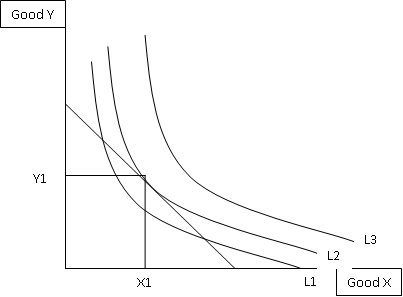
Next, we'll move on to a more complex concept - the optimum consumption point! This is where we combine the budget line from above and the indifference curves from the blog post I did a few days back. By definition, the optimum consumption point will be where the budget line touches the highest indifference curve on an indifference map. As with most concepts, this is also much easier to understand when represented on a diagram:

Here you can see that the budget line touches, or is tangential, to the indifference curve L2, which is the highest one it touches. Therefore we can say that the optimum consumption point for these two goods would be X1 of good X and Y1 of good Y. We know the slope of the budget line is Px / Py and we know from the previous blog post that the indifference curve slope at any point is MuX / MuY. Therefore, the optimum consumption point is the point where (Px / Py) = (MuX / MuY)!

A change in income will cause a change to the diagram. The budget line will either shift out or in depending on whether incomes rose or incomes fell. This new budget line would cross and indifference curve at a different point, if you joined the new optimum consumption point and the old one you'd have created a new line that we call the income-consumption curve in economics. As with a change in price of one of the goods, the budget line will pivot and a new optimum consumption point will be formed. Connect the original point and the new point and this line you've created is called the price-consumption curve. 

Now for the exciting bit! Actually deriving a consumers demand curve for a good!  


Ok, there is a demand curve derived for good X using the indifference curves and budget lines. Look at it, take it in, see if you can see what's going on. It's difficult, I know. Here's my explanation attempt: On the top diagram we have used good X along the bottom and money for all other purposes on the Y axis. We have a set budget and at varying prices of X this budget line is pivoting. Each of these new pivoted budget lines crosses indifference curves at different points to form a price-consumption curve. The points of intersection of each budget line translate down to as the quantities demanded of good X. Now, to work out the prices for the second diagram. Lets look at the first budget line for this. It crosses L1, we can see that. At that point it has translated down to the bottom diagram as Q1. The price here is the same as the slope of the curve.. so assuming we have a budget of £30 I'd say the budget line hits the X axis at roughly 17. So, 30/17 = 1.76, which is the roughly where the point is on the second diagram. If we did the same for the other two budget lines we'd receive prices of 1.2 and 0.94. These are those two other price points you can see on the diagram. Then as with any other demand curve, join the dots to actually complete the demand curve for good X. PHEW!

That's it, finally. It may be difficult to grasp in parts, if it is then comment with where you are finding it difficult and I'll give you a helping hand. I'll get back to you within a few hours normally, so keep checking back! Thanks for reading again guys, have a good day.

Sam. 


Monday 15 October 2012

'Dilemmas of an Economic Theorist'

Just a quick one here, thought I'd pass on a link to a great article I've just read by Ariel Rubinstein. He's written a paper named 'Dilemmas of an Economic Theorist' in which he questions the place of economists in the real world. Whether our models and our input are actually having a positive impact on the real world. It's a very engaging and entertaining read, much different from your standard academic paper. The conclusion is that the models we economists create are much like fables or fairy-tales as we make our models free of extra data and annoying diversions, just like in a fable. Have a read, here's the link:


Let us know what you think of it. I'll be back later in the week with another post, so have a good few days! Cheers guys.

Sam.

Friday 12 October 2012

Preferential Trading Arrangements

Preferential trading arrangements refer to such things as trade blocs. Trade restrictions are held with the rest of the world but lower restrictions or none with member states. There are three types of preferential trading arrangement:

  • Free Trade Area - This is when member states remove tariffs and quotas with one another. However, restrictions on trade with non-member states are kept individual to each nation.
  • Customs Union - This is the same as above, but in addition there are common external restrictions on trade with non-member states. 
  • Common Markets - This takes it one step further and the members operate as a single market. This means as well as the features of the above arrangements there is also a common taxation system, common laws regarding production, employment and trade, free movement of labour and capital and no special treatment by governments to their own domestic industries. Additionally to this, we sometimes see fixed exchange rates between members and common macroeconomic policies. 

Next we move on to trade creation and trade diversion, which come as a result of preferential trading arrangements. First, trade creation. This is when consumption shifts from a high-cost producer to a low-cost producer as a result of of joining the customs union. Normally this is due to obtaining the goods cheaper from other members of the union. As with most things, this can be modeled on a diagram! 

Trade Creation Diagram

This is it, the trade creation diagram. Let's explain it a bit. SDom and DDom are the domestic supply and demand of a good. Before the EU, the country had to pay at the 'PEU + tariff' price so domestic production was at Q2 and domestic demand was at Q1. The imports here were the difference between Q1 and Q2. With the joining of the EU, the price was now the PEU price, lower than before. This meant domestic supply had fallen to Q4 and domestic demand had risen to Q3. So the new imports level is the difference between Q3 and Q4, which is higher than before. Thus, trade has been created. 

Trade diversion works in very much the opposite way. This is when consumption shifts from a lower cost producer outside the customs union to a higher cost producer inside it. There is a net loss in world efficiency now the higher cost producer is being used. 

Trade Diversion Diagram


This is the trade diversion diagram. The country was initially paying price P1 for the good, meaning they consumed at Q1 and produced at Q2. Price falls to P2 because of the joining of the EU. We can see here, that consumer surplus has improved. The original consumer surplus at price P1 has now increased to include the areas 1, 2, 3 and 4 on the diagram. We also notice a loss of producer surplus by area 1 which will be the fall in profits. No tariffs are paid out anymore, so the areas 3 and 5 are lost to the government in terms of revenue. This leaves an overall net gain of areas 1 + 2 + 3 + 4 - 1 - 3 - 5 = 2 + 4 - 5. Here we can decide whether the trade diversion has been beneficial or detrimental. If the size of area 5 which we have lost is greater than the size of areas 2 plus 4 which we've gained then there is a net loss, otherwise we've achieved a net gain. 

If there are high external tariffs or a small cost difference between goods produced inside and outside of the union then a customs union is likely to lead to trade diversion.

In the long term, a customs union could have advantages and disadvantages, I'll name a few of both:
  • Advantages:
    • Increased market size - allows firms to potentially exploit economies of scale to lower costs.
    • Better terms of trade with world markets because of the power of the customs union.
    • Increased competition which will stimulate efficiency and bring costs down.
  • Disadvantages:
    • Resources may flow to the geographical centre for the lower transport costs leaving depressed regions on the edge of the union.
    • Mergers will be encouraged which will boost monopoly powers.
    • Diseconomies of scale.
    • The administration costs of maintaining the union.

The basics of preferential trading arrangements in one blog post, tadaaa! Thank you for reading, keep sharing and following the blog! Thanks guys, have a good day.

Sam.