Factor Markets

When discussing factor markets we are talking about the market for factors of production. Recall the circular flow of income (there is a post on it somewhere) - firms are demanders of factors of production and households are suppliers. Firms pay money to households in exchange for their factors of production - wages for labour, for example.

We'll be looking at perfectly competitive factor markets. Everyone in this market is a price taker, whether it be the firms, the workers or whoever. Freedom of entry and exit exists. It costs nothing for a person to leave the labour force and nor does it cost anything for someone to join it. We assume that the factors are homogenous. Everyone/everything in the market has the same level of skill and motivation. Finally, there is perfect knowledge. Workers know everything about the firm and firms know everything about the workers, for example.

Let us zoom in on the labour market more specifically. A perfectly competitive labour market looks as follows:

On the left we have the market as a whole. The wage rate is determined by the interaction of demand for workers and the supply of workers.  With this wage rate, we can look at an individual firm on the right. At wage rate W the firm would be willing to employ Q hours worth of labour.

We need to somehow ascertain how much labour would be supplied by people in the labour market. This figure is dependent on many factors. From the point of view of the worker, working involves disutility's such as sacrificing leisure time and it being tedious/boring.  The more they work the larger the disutility. The marginal disutility of work (MDU) will increase as people work more. Due to this, we see an upwards sloping supply curve of labour. To encourage people to work more hours, higher wages need to be paid in order to compensate for the higher disutility.

In general, an individual's supply of labour will look like this. The higher the wage rate, the more hours worked. However, there is a case where the shape of the individuals supply of labour actually bends backwards. This is the case when an individual feels that after a certain point they can afford to work less and have more leisure time. It looks like this:

Once wage reaches W the individual feels that they are earning enough and can afford to cut back on the amount they work should wages rise further.

The amount of labour a firm demands rests on the assumptions that firms are trying t maxisimise profits. The theory is known as the marginal productivity theory. We look at the marginal revenue product of labour in this piece of analysis (MRPL). We know that to maximise profits, marginal costs must equal marginal revenue, so therefore the firm will employ labour up until the point wages (the marginal cost) equal the marginal revenue product of labour. It looks like this:

The firm will hire Q hours worth of labour in order to maximise their profits. What about the demand curve for a firm as a whole? Well, because whatever the wage the firm will be producing where wages equal MRPL, this means that the demand curve for the firm is the MRPL curve. From the peak of the curve to the right is the demand for labour for a firm trying to maximise its profits.

There are some firms that are known as monopsomists. These firms are wage setters, not wage takers. They are a firm with monopoly power on factors of production in an area - say a single employer in a village. They have the power to restrict the amount of labour they employ to keep wage rates down. The firm faces an upwards sloping supply curve for labour, to employ more workers they need to pay a higher wage rate. This supply curve shows us what wage must be paid to attract a certain amount of labour. The wage is also the average cost of employing labour, therefore the supply curve is the AC curve. The marginal cost of labour will be above the average costs because to attract more employees the wage rate must be raised. The profit maximising point for the firm would be where MCL = MRPL with a wage of W1. If we were in a perfectly competitive market the wage rate would have been at W2 with a higher amount of labour employed. The monopsomist forces the wage rate down by restricting how many workers it employs.

Monopoly, Monopolistic Competition and Oligopoly

Before we look specifically at any of the three market structures in the title we should take a closer look at revenue as this will be important in the analysis. When price varies with output, which it does in all market structures bar perfect competition, the demand curve is downwards sloping. Average revenue equals (total revenue) / (quantity). This is the same as (price x quantity) / quantity. Cancel out the two quantities and we're left with average revenue being equal to price - hence it is equal to the demand curve.

So, the average revenue curve is sloping downwards because it is equal to price. Why the position and shape of the marginal revenue curve then? Well, as we know, marginal revenue is equal to the change in total revenue divided by the change in quantity. If we substitute in price x quantity for total revenue we are left with: 

If we use the product rule to differentiate this (Google this or find a text book, I'm not going to explain the pure math behind it) we're left with marginal revenue being equal to: 

The change in price over the change in quantity will give us a negative figure, so what we're left with is Price + something negative. Due to the "+ something negative" it will be falling below the AR curve, hence its position on the diagram above.

The total revenue curve interacts nicely with the marginal revenue curve we can see above. The total revenue curve increases at a decreasing rate. Why? Well, because to sell more the firm has to lower its price. Due to this, there will come a point when total revenue is maximised. This will coincide with the quantity at which marginal revenue is equal to 0. That quantity will be the revenue maximising quantity for the firm.

Now that we've understood the concept of revenue, let us hone in on the specific market structures. We'll start with monopoly. In a monopoly we have one firm that dominates the market. How do they do this? It is largely due to the barriers to entry into the market. They could be any of the following:

·         Economies of scale.

·         Legal restrictions.

·         Aggressive tactics.

·         Product differentiation.

...the list does go on. These all make it very difficult for new firms to break into the market and pose any sort of competition/threat to the existing monopoly firm. Graphically, a monopoly looks as follows:

They produce at the point MC = MR because this is where profits are maximised. At this point there is a difference between average costs and average revenue, revenue exceeds costs which means that the monopoly is making a supernormal profit. All pretty obvious thus far. Monopoly is probably the easiest of the market structures to master, all there is to remember is that supernormal profits are made in the long and in the short run. To the consumer a monopoly may seem to be a disadvantage - higher prices and lower output compared to perfect competition. This is true, but it does have its advantages. Firstly, supernormal profits fuel innovation which can lead to better, cheaper products in the long run. Secondly, if the economies of scale are big enough then through a monopoly some markets can exist that wouldn't be possible if monopolies weren't allowed. This is in the case of a natural monopoly.

Natural monopolies are markets that have very high, fixed  start-up costs. So high that it becomes unprofitable if more than one firm try and provide the good/service. An example would be the London Underground - massive start up costs in laying the foundations of the network. So, if there were two firms in the market a loss would always be made and therefore production wouldn't occur at all. See this diagram below.

If there was two firms trying to run versions of the Underground simultaneously then neither would be able to stay afloat only serving half of the market each - whereas one firm serving the whole market means it is affordable. With two firms, the demand curve above with slope down at twice the rate meaning it is always below the long run average costs curve, meaning a loss will be made. The scale of production that comes with a natural monopoly means that costs can be lower and therefore the market price can be something consumers will be willing to pay.

That's the low down on monopolies. Now to move onto monopolistic competition. Do not get the two confused - similar names yet totally different market structures. In a monopolistic market firms sell a different variety or different brand of the same product. There are many firms that all act independently of each other with freedom of entry and exit into the market. There is symmetry in the market - new firms entering the market effect all old firms equally.

1 = Firm demand. 2= Firm demand after new competitor enters.

Each firm has a share of the whole industry, but can only influence the price minimally, hence the inelastic demand curve for the firm. Every time a new firm enters the industry all existing firms will see their demand decrease and the influence they have on industry price fall. Every new firm that enters moves the market closer to perfect competition.

A firms profit in the short run looks strikingly similar to that of a monopoly. Supernormal profits are available. However, emphasis on 'short term'. Over the longer term more firms enter and prices are forced down. The quantity each firm supplies is also forced down and supernormal profits are quashed. Firms will keep entering until average costs equal average revenue, at this point no more supernormal profit is available. We haven't entered perfect competition because the demand curve/average revenue curve is sloping downwards meaning price is not constant across all firms.

On the left we have the firm in the short run. Supernormal profit is made. The new firm enters and we move to the situation on the right hand side. The firms individual demand has fallen, and thus its average revenue and marginal revenue have fallen too. This means that the amount of profit that is made has fallen. These firms will keep entering and this will keep happening until supernormal profit is wiped out completely.

The model is all well and good taken at face value - but it does have its limitations. In reality there is imperfect information about profits and demand, it doesn't take into account the effect non-price competition has and in reality it is difficult to identify an industry demand curve. Bar all of these problems it does give us a fairly accurate representation of a monopolistically competitive market. One problem with this market type is because of the downwards sloping demand curve - production will not take place at the lowest long run average cost. Therefore monopolistic competition isn't as efficient as perfect competition.

The final type of market structure to analyse is that of an oligopoly market. Oligopoly is when there are a few large, major players in an industry. 3 or 4, for instance. There are significant barriers to entry and firms are very interdependent. The firms have to look at the incentives to compete with the other dominant firms and the incentives to collude with these firms to determine their plan of action.

Now, to determine the total production of an oligopoly market we have to run through a little story. We start with an industry with one firm acting as a monopoly. The firms demand function is as follows: P = 200 - Q and its marginal costs are 0.From this, we can see that if quantity was 0 then price would be 200 and if price was 0 then the quantity would be 200. We can use this to draw an initial demand curve.

We derive the marginal revenue curve by differentiating total revenue. Total revenue = (200-Q) x Q, and that differentiated leaves us with: MR = 200-2Q. Profit is maximised at MC=MR, and MC = 0, so therefore the firm will produce 100 of the good. Half the market is supplied.

Now, the next part of the story is for a competitor to enter the market. Firm B spots that there is unfulfilled demand, 100 of it, and decides to enter the market. The demand curve for Firm B is going to be: P = 100 -Q. With that as the demand curve, and using the method in the paragraph above, firm B works out it's marginal revenue curve to be: MR = 100 - 2Q. The new market now looks like this:

Firm A is still supplying 100 of the market and now Firm B has entered and is supplying an additional 50 to the market. 150 of the market demand is satisfied.

But, the next day Firm A reacts to this new firm. They have to readjust and now see their demand function as: P = 200 - Q - 50, or P = 150 - Q.

Both Firm A's demand and MR curves have swung in, and now it finds itself supplying only 75 to the market compared to the 100 it was supplying previously. The new entrant has brought down Firm A's production. 125 of the market is now supplied.

Firm B has to react to this change from Firm A. It sees Firm A's new supply of 75 and recalculates its demand function to be: P=200 - Q - 75, or P = 125 - Q. From this it gets its marginal revenue to be: MR = 125 - 2Q. At this marginal revenue Firm B will now increase its production to 62.5. 137.5 of the market demand is now satisfied. You may have noticed some repetition here. The market will keep going back and forth between the two until an equilibrium is achieved. Firm B's production increases whilst Firm A's falls. So when will equilibrium occur? It will be the point when one firm reacts to another firms level of supply and achieves the same level of supply. In the example above this is when 66.66 is produced by each firm, leaving the 133.33 of the market demand being satisfied.

What we have described above is typical when the number of firms in an industry is small - it is known as Cournot competition, competing over market share. As we see above, with 2 firms in the market each firm supplies 1/3 of the total demand in equilibrium meaning 2/3 of demand is satisfied. With 3 firms in the industry, each firm will supply 1/4 of the total demand in equilibrium meaning 3/4 of demand is satisfied. Each additional firm added means more of the total demand is satisfied and therefore the market is moving closer to perfect competition.

What can we say about profits under Cournot competition? Well with the total demand function being P = 200-2(Q) we can calculate price to be 66.66 by substituting in the equilibrium quantity we derived earlier. We assumed costs are nothing, therefore total revenue in the industry will equal 2(66.66 x 66.66) = 8887.7. Sounds like a nice figure. However, what would it be under a monopoly? We saw Price and quantity equal to 100 when there was just one firm, so total revenue will be 100x100 = 10,000. Higher than in the oligopoly. This tells us that firms would be better off if they got together and agreed to limit the market - this is known as collusion.

Collusion can happen in many ways, one of these being price leadership by the dominant firm. In this scenario, the dominant firm makes an assumption that all the smaller firms in the industry will act like a firm in a perfectly competitive market once it has set the price and chosen its output.

The dominant firm has to decide the price it is going to charge. The price has to be between the range of P1 and P2 above. Any higher than P1 and there will be excess supply, any less than P2 and they won't be able to afford to supply anything. So, the demand curve for the dominant firm runs from P1 down to the point on the market demand curve that coincides with P2. So, the leader can choose a price, say P. Then, with a price decided the dominant firm has to decide how much it will produce at this point and therefore how much of the market is left for the other smaller firms.

So, Price P was decided by the leading firm. Therefore, at this price the dominant firm will supply QL to the market (Where P = Dominant firm demand). The following firms will supply QF to the market (Where P = S) and the total supplied to the market will be QT. QT should be QL + QF. That is one form of collusion between firms - a very subtle one and therefore very difficult to prove.

A few rules of thumb are used when it comes to tacit collusion - using an average cost mark-up when it comes to pricing, for example. Something like P = (1 + 0.1)AC would do the trick. Firms would agree on a certain rate of profit and then enforce this pricing mark up to achieve that. They also use benchmark pricing, £9.99 or £14.99 for example.

As far as collusion and the law goes it's a tricky one. It is illegal but it can be incredibly difficult to prove that it is actually going on. It is entirely up to the authorities to decide the difference between prices being set competitively and firms agreeing prices. Unless it is really bad or really obvious it rarely gets proved.

Phew, that is it. Cheers for reading guys. Same script - comment if you need any additional help or you spot mistakes, all feedback is welcome!

Sam.

Perfect Competition

Perfect competition is a very unrealistic market structure. We'll discuss the characteristics of it later, but for now we have to understand that it is a theoretical concept. If the world was perfect then in most cases we'd have markets operating 'perfectly'. The world isn't perfect and therefore actually seeing perfect competition in reality is a long shot. The major assumption we make is that firms are price takers. By this we mean that each firm alone has no influence over the market price because of their relative size. They take the price they can get as given and perceive it to be constant. Therefore the demand curve for a firm in perfect competition is horizontal - the can sell as much as they want but only at the market set price. Any higher and they wouldn't sell a thing, any lower and they'd make a loss in the long run.

Here we have a typical perfect competition scenario in the short run. On the left is the market where the market price is determined by the supply and demand for the good. The firm, on the right, takes the market price as given and as their price. Average revenue and marginal revenue is the same as the demand curve because we are looking at a constant price for the good. Production takes place at the point where MC = MR, anywhere before this point and more profit can be made, anywhere after this point and profit falls. If you look at the diagram, at the point MC = MR, the average cost is below the average revenue. This means profit is available, which is shown by the yellow area. In the short run the supernormal profit will be (AR-AC) x Qe.

Now, above I've just said that AR and MR are the same as demand because price is constant. You want proof I hear? Sure thing. Average revenue = Total revenue / Quantity. Total revenue is actually price x quantity. Therefore average revenue can be re-written as (price x quantity) / quantity. Quantity cancels out leaving price ~ average revenue = price. Marginal revenue = the change in total revenue / the change in quantity. Substituting in what total revenue actually is we have the change in (price x quantity) / change in quantity. The change in quantity cancels out leaving price ~ marginal revenue = price. Boom!

But, we have only discussed the short run. These supernormal profits don't go unnoticed - they attract new firms into the industry. Supply now shifts out.

The price falls due to the increase in supply. On the right diagram we can see that it's fallen to the point where MC = MR = AC. This means that supernormal profit is no longer being made, it has been competed away. At this point no more firms will enter the industry because there won't be the pull of supernormal profits. Therefore, in the long run there is no supernormal profit to be made in a perfectly competitive market.

It seems risky to the normal person, producing right on the point of breaking even. This is true to a certain extent. Shocks to the system could cause demand to fall, what would happen to the firm then?

Here we have the case of a fall in demand in the market causing a fall in price. The firm was initially producing where MC = MR = AC, but now the fall in price means that if they produce at MC = MR they will actually be making a super-normal loss. This point would be below average costs and therefore the enclosed area on the right hand diagram would be loss. Would they carry on producing? Surprisingly, yes, in this case the firm would. To understand this we have to look at the breakdown of the costs. In the short run we know capital is fixed and labour is variable. Therefore the average variable cost for the firm in a simple world would be labour costs / quantity. As long as the average revenue (demand curve) is greater than the average variable costs then the firm will continue producing. This means they can cover the costs of labour and make some contribution to the fixed costs. If they couldn't cover the average variable costs it would be better for the firm to stop producing, lay off all the workers and only lose the fixed costs.

Some other things we can state is that the short run supply curve for a firm in a perfectly competitive market is the marginal cost curve until the point where price equals average variable cost. As we said above, below that point the firm will stop supplying the market. In the long run the firms supply curve is horizontal at the minimum average cost.

All we need to do now is sum up whether perfect competition is a good thing. It definitely has its advantages, they are as follows:

·         It's efficient - production occurs at the lowest average cost which is the most efficient point.

·         Competition - competition in an industry forces firms to be more efficient.

·         Price is influenced by demand - the market is essentially run by consumers, it responds to their behaviour.

·         No supernormal profits in the long run.

It really has few disadvantages though. You could state the fact that it isn't realistic as a disadvantage, I guess. In real life it would be rare to find a market with freedom of entry/exit, identical products, price taking firms, etc. One point that could be made about the lack of super-normal profit is the lack of innovation. Innovation tends to be fueled by profit, without profit there is little room for firms to innovate. Innovation is one thing that can lead to a more efficient market, so in perfect competition once the efficient point is reached it will not be made any more efficient. Comprende?

Sam.

Indifference Analysis

Back to a more educational point of view now following the last post I wrote. Today will be a look back, potentially in more detail, at the concept of indifference analysis. I'll try and start at the very basics and work my way through the subject - if you feel I've left anything out do not hesitate to let me know in a comment and I'll try and go over it for you. This post is long, I won't hide that fact. Make full use of the search bar to the left of this to make sure this contains what you're looking for. Even better still, use Ctrl + F and search for keywords. That could save you some time!

Indifference analysis is a basic concept in economics which looks at consumers preferences for two goods. It is an "exactly what it says on the tin" topic - we are looking at combinations of these two goods that the consumer would feel indifferent about. The definition of 'Indifferent' from dictionary.com, by the way, is "having no bias, prejudice, or preference; impartial; disinterested." So, rephrasing it into Layman's terms: we are looking at combinations of these two goods that the consumer would feel equally as happy, content, etc with. This will become evident later on in the analysis.

The very first step in the analysis will be to construct an indifference curve. This is done below.

Here we have an indifference curve. This is modelling different combinations of Good A and Good B that the consumer would feel indifferent about. Anywhere along this curve the consumer will be feeling the same level of satisfaction. Indifference curve slope downwards - that is a general rule. Why? I hear you ask. Well, it's due to the diminishing marginal rate of substitution. This piece of jargon essentially means the rate at which we would swap Good A(Y) for Good B(X) while remaining equally as satisfied. It looks as follows:

                                               
If we used some figures as an example, let's say that the consumer is indifferent between 25 of Good A and 5 of Good B and is also indifferent between 20 of Good A and 6 of Good B. Right. So, the top of the equation would be (20 - 25) and the bottom of the equation would be (6 - 5). That leaves us with -5 as the answer. So, between the points (25,5) and (20,6) on a diagram the slope would be -5. We can focus in on the negative sign here, this shows why the curve is always downwards sloping. We have to give up some of Good A to get more of Good B. Keeping up? Good.

An indifference curve alone tells us very little, an indifference map on the other hand tells us a lot more. An indifference map is a series of indifference curves showing which combinations of two goods give different levels of satisfaction.

If you think of the map as a mountain, starting from the bottom left corner and working diagonally to the right and up - the higher up the mountain we go the more satisfied the consumer. At any point on I4 the consumer is more satisfied than at any point on I2 for example. The question that creeps up a lot regarding indifference curves is "Could they ever cross?" In short, the answer is no. This can be proved via contradiction.

Consider the three points here: a, b and c. From the analysis we've just done we can say that a is indifferent to b. We can also say that a is indifferent to c. So, b 'should' be indifferent to c. But b has more of Good A for the same amount of Good B than c does, and therefore point b would be preferred. b and c aren't indifferent, and therefore indifference curves cannot cross. Bosh!

Now, for a consumer to make a decision about what to consume we need more information than just the indifference curves. We need information on prices and incomes. This is where the budget line enters. I fear I'm stating the obvious here, but I'll have to continue: the budget line is how much of the two goods the consumer can afford. So, it'll have the following formula, which reads 'Price of Good A times the quantity of Good A plus the price of Good B times the quantity of Good B equals the consumers income:

If Good A was £2,  Good B was £1 and the consumer's income was £30 then we'd have an equation to work out: 2A + B = 30. Now we have our equation we can plot the budget line on a graph.

It is literally as simple as that for the budget line. All we need is the price of the two goods and the consumer's income and we can work out the quantities of each good they can purchase. While on the topic of the budget line I think I'll mention what happens to the line when prices and incomes change. If just one price changes then the budget line will swing in or out, pivoting around a point. For example, if the price of Good B fell, then we'd see the line swing out to the right, pivoting around the point on the Y axis. It would swing out because a fall in price of Good B means we can afford more of them. A rise in price causes a swing in. A change in the total budget or consumer's income means a shift in the whole budget line parallel to the current one. A rise in the budget shifts the curve out to the right, a fall in the budget shifts it in to the left. If both incomes and prices rise by the same percentage, or fall by the same percentage for that matter, we see no change in the budget line.

Moving swiftly on, we're ready to combine the indifference map and the budget line. This can give us the consumer's optimal consumption point. Utility or satisfaction for the consumer is maximised at the point of tangency between the budget constraint and the indifference map, as is highlighted in the graph below.

The slope of the indifference curve is the marginal rate of substitution and the slope of the budget constraint is (minus) the relative price of Good A and Good B. Therefore, where these meet, the consumer chooses optimally when MRS = Price of Good B / Price of Good A.

Another piece of jargon you may need to learn is the 'Price-Consumption curve'. This is a curve derived from the changing price of one of the goods. From this curve we can create a demand curve for that good. Clever stuff.

Now, to derive the demand curve from it. We make one alteration to the diagram above, we make the Y axis 'Expenditure on all other goods' instead of just Good A. Then, we follow the points of tangent down and onto a new diagram. On the Y axis of the below diagram we list the prices, which come from dividing the Budget by the quantity of Good B when expenditure on all other goods is 0. Match these prices up to the lines we've just drawn down and Bob's your uncle - a demand line. In words it sounds confusing, take a look at the diagram below and then re-read this until sense is made.

I hope that makes sense - reread and study the diagram.

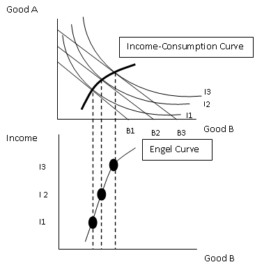
Another 'special' curve we need to be aware of is the Income-Consumption curve. This tracks the effect a change in income has on our optimum choices of the two goods. The slope of this curve tells us about the desirability of Good A and Good B as incomes rise. In general, the curve will look something like this:

There is a special case where the shape of this curve bends the other way. This is when one of the goods is an inferior good - I trust we all know what that means. A higher budget will mean less is demanded and therefore the income consumption curve will bend back on itself.

Bravo to those of you that have made it this far and hello to those that skipped straight to this section. Neither of you will be judged... honest. Finally, we are going to look at the Engel Curve. An Engel Curve shows how the demand for a good changes as income changes. We use the Income-Consumption curve and track it down onto a new diagram below.

If incomes increase and this leads to a demand increase for the good then we are looking at a normal good. If demand decreases it is an inferior good. The final, more peculiar outcome, is in the case of a giffen good. Giffen good prices rise when demand rises, odd - but they do exist.

By gosh, I think we might be finished. I said 'potentially' more in depth at the beginning - I think that word can be scrapped. If you're still unsure of anything Indifference Analysis related then drop me a comment and I'll be happy to try and help you out if I can. Thank you for reading, have a good day!

Sam.

Principles of Economics - Perfect Competition

Perfect Competition is a market structure that follows these assumptions:

• Firms are price takers - each firm has no impact on the price in the market, they take the price the market forces set.
• Freedom of entry into the market - there are low barriers to entry so anyone could potentially set up in this market.
• Firms produce identical products - the taxi market for example, each taxi firm offers an identical product.
• Producers and consumers have perfect knowledge - both producers and consumers know everything there is to be known about the market.

However, few, if any, industries are actually perfectly competitive.

In the short run, the number of firms is fixed. In the long run, if supernormal profits are being made then new firms will enter the industry. If losses are being made, firms will leave the industry. 

Short run equilibrium of the firm:

This is what the market looks like in the short run in perfect competition. The price is Pe, and is set by the demand and supply forces. It is horizontal because firms are price takers. Due to price being constant, the red dotted line is also the average revenue, the marginal revenue and the demand for the firm as they're all the same. Qe is the amount produced by the firm because this is the amount at which profits are maximised (MC = MR). There is slight profit being made because the average revenue is higher than the average cost at the production point.

This is where the long run can be introduced. In the long run, firms see these profits being made and enter the industry. These means the industry supply increases, shifting the supply curve to the right on the left hand diagram above. Price falls, which means each firms demand falls until the point it is equal to the average cost. At this point, firms break even and make no profit. Firms will stop entering the industry now.

As far as the public interest goes with perfect competition, it has its benefits and drawbacks. The benefits are as follows:

• Firms produce at the least cost output.
• Firms that are inefficient will be forced out.
• Prices are minimised.
• Consumers determine what and how much is produced.

The drawbacks are:

• There us very little incentive to invest in new technology.
• Goods are all the same, lack of variety for consumers.

That ties up this post about perfect competition. Thank you for reading, keep checking back and sharing. Have a good day!

Sam.

Common Agricultural Policy Part 2 - Declining Farm Incomes

The next thing the CAP aims to eradicate is declining farm incomes. These are mainly caused by two things: low income elasticity of demand and/or increases in supply. As usual, we'll display this diagrammatically. Lets suppose we have a fairly inelastic demand curve and at the same time farm efficiency has improved, we can expect the market to now look as follows:

We can see that prices have fallen from P1 to P2 and quantity has risen from Q1 to Q2. However, we can also see that this has caused a fall in income of area a and an additional income of area b for the farmers. Area a is clearly larger than area b, meaning the farmers income as a whole has fallen. The way for farmers to gain is for demand to shift out by a larger amount, as even a small shift in demand would leave farm incomes still falling. 

What the farmers need is a more elastic demand curve for any increases in supply efficiency to actually increase farmers income. However, demand for grown crops is generally more inelastic because it's a necessity and therefore a change in price really doesn't affect demand all that much. This is why the government needs to intervene with the CAP because else there would be no incentive for farmers to make their production mechanisms more efficient as they'd effectively be losing money due to it.

Now we have covered both reasons as to why the CAP is necessary; fluctuating crop prices and declining farm incomes. We will next cover how the EU uses it's policies to correct these issues. Stay tuned!

Sam.

Common Agricultural Policy Part 1 - Price Fluctuations

The Common Agricultural Policy is a massive deal in Europe and the European Union. It's a very expensive policy that started out back in 1962 as a simple price support policy. It has two key objectives: to stabilise prices and to provide income support for social reasons. If you look at the distribution of farms across Europe, it is clear to see why this is needed. The biggest 7% of farmers own roughly half the land, whilst the smallest 50% of farmers own only 7% of land. This is a massive inequality and could lead to monopoly powers, outlandish prices and other such problems if it went unregulated.

We'll first look at a few of the characteristics of the agricultural industry. There are many producers, all are price takes. There are also many consumers, all of which are also price takers. There is generally freedom of entry and exit into the industry. It's about as close to perfect competition as you could get in a realistic scenario. Governments need to intervene for many reasons:

• To reduce price fluctuations.
• Raise farm incomes.
• Protect rural communities.
• To encourage greater self-sufficiency.

Firstly, I'm going to focus on the price fluctuations. In the short term they are caused by instability and the fluctuations in the harvest (good or bad!). Let's assume that the demand for a crop were to rise one year, which would cause a shift to the right of the demand curve. Supply in the short term obviously cannot react to this because supply is fixed each year depending on what is planted. This demand rise will cause a rise from price P1 to P2. This is all shown on the diagram below.

The farmers observe this rise in price and then next year they increase their supply to the market. At P2 the farmers decide that Q2 is the correct quantity to supply to the market. However, at this amount supplied, demand is outstripped and therefore price must fall to P3. The year after, at price P3 a different amount is supplied by the farmers, but at this supply more is demanded and therefore price rises again. This will continue, as shown on the diagram below we can see that the market is slowly spiralling towards a point of equilibrium at which both consumers and producers would be happy. 

We call this concept a stable cobweb. This price fluctuations and changes are supply are making the market more and more stable as over time the fluctuations get smaller until equilibrium is finally met. In this case, the government wouldn't need to intervene in the agricultural industry. However, there is the opposite case. An unstable cobweb could appear. The case of this occurs when the supply of the crop is very elastic. Diagramatically, the supply curve will be much flatter. The same instance as above will occur, demand increases causing a price rise as supply is fixed. In the second term supply is increased due to this new price, but there is oversupply and price has to fall... and so on and so forth. Except, when the supply curve is elastic this doesn't spiral towards equilibrium, it spirals away from it as can be seen in the diagram below.

This shows one of the cases in which the government would need to intervene in the agricultural industry, hence the Common Agricultural Policy. The price fluctuations in this unstable cobweb would keep getting worse and worse if left to market forces. 

Next we'll move on too supply side shocks. This is when supply is affected, either for good or for bad, and therefore the supply of the crop isn't as expected. Once again, diagrams are an easier way of showing this. The first case will be a bad harvest, where supply of the crop is less than what was expected. The diagram below shows this. Supply of the crop has fallen from the expected level of Qe to the actual level of Qa. The area labelled 'b' is income that the farmer has lost, the area labelled 'c' is income gained from this supply side shock. The expected income for the farmer was area 'ab', but the actual income of the farmer is now area 'ac'. If area c is greater than area b then the farmer has gained, otherwise the farmer has lost out due to the bad harvest. Generally, the more inelastic demand is, the greater are 'c' is and therefore the more likely the farmer will benefit. 

I'll quickly go through the other supply side shock as well. As you can guess, this is when there is a better harvest than expected. This causes a shift to the right of actual supply from Qe to Qa. A fall in price is seen from Pe to Pa and once again the farmers income may be affected. Area 'c' is the income gain, area 'b' is the income loss and area 'a' is the income that has stayed constant. If area 'b' is bigger than area 'c' then the farmer has lost out. 

What we have achieved in this blog post is the causes of the fluctuations in prices of harvested goods. This is one of the things the Common Agricultural Policy aims to stop, as stable prices is an aim. In the next post we'll look at what is causing the decline of farmers income and then we'll move on to look at how the government intervenes in this policy to correct these issues.

Stay tuned guys, enjoy!

Sam.

The Transformation of Policy Between the Wars

Immediately after the First World War, the government's aim for policy was to get the economy back to the 'normality' experienced prior to 1914. This sort of thing included the government playing a limited role in the economy, more integration with the world economy and restoration of the gold standard, free trade and a balance budget.

Initially these three final points are achieved. The budget is eventually balanced, albeit a higher budget than previous years due to the increase social spending and maintenance of the national debt. During the 1920's the policy of free trade is also pretty much restored. Britain gets back on the gold standard in 1925 at the rate of £1 = $4.86. Germany and France both rejoin the gold standard at a similar time, along with most other leading economies. Why did we return to the gold standard you may ask? Well, firstly it helped achieve the restoration of pre-war 'normality'. Also, it aimed to try and stabilise the currency which would in turn help out trade. Another feature of the gold standard was to allow the monetary system to function on its own. What I mean by this, is that if the country runs a payments surplus then gold will flow into the country, interest rates will be decreased so wages and prices will fall. This will in turn cure the surplus. It also works the opposite way for a payments deficit. A final point is that the gold standard was a means of stopping politicians from meddling with the money supply!

However, pre 1914 the gold standard worked but after the war and during the 1920's it just didn't. There is a list of potential reasons for this:

• Why the gold standard worked pre-1914:
• It was developed gradually over time.
• Capital and labour was freely moving.
• The central bank could use interest rates to protect the currency, independent of the government. 
• London was still a financial centre.

• What changed in the 20's?
• There was a rush to return to the gold standard.
• More protectionism and less migration due to barriers.
• Central banks were under pressure from politicians.
• Paris and New York now competing against London as financial centres. 

Mr. Keynes pops up again in this debate. He pointed out that British prices had risen faster than the US', so starting at the same £1 = $4.86 rate would be an overvaluation of the pound. Although this shouldn't have matter because the gold standard should re-adjust prices, Keynes doubted it would work. He thought it would have bad domestic effects including interest rates needing to be kept at 4.5-4.5% and due to this borrowing would become expensive and investment would suffer.

The world slump is the next chronological step in the economic history of Britain. The recession of 1929 - 1931 started because of the Wall Street Crash in the US. This meant massive balance of payments problems. In 1931 came the European Banking Crisis and so in Autumn of that year Britain was forced off of the gold standard. This was first portrayed as a temporary change, but gradually the realisation came about that it was for good. Interest rates were cut to 2% to encourage borrowing and investment which would boost the economy again! Amazingly, there was a recovery. GDP rose as investment rose and Britain actually now compared well with other global economies. It would be easy to say all of this was because of the gold standard, but it isn't true as many other factors were also contributing to the recovery of the British economy. What the slump did cause, however, is the abandonment of free trade between 1931 and 1932. 

Keynes had the idea that investment from the government was something that was necessary for the economy. But, the treasury wasn't in agreement with this theory. They believed it would unsettle foreign investors and worsen the national debt. Keynes thought that there was no point in cutting wages because demand and consumption would suffer. What was needed was public investment which would boost the economy via the multiplier effect. The treasury argued it would be inflationary and any more borrowing would get out of control. The only time borrowing was allowed was in a one-off circumstance for rearmament!

Thanks for reading again guys, that'll be it for economic history for a while... I promise! Haha.

Sam. 

The Role of the State and the Challenges of WWI, 1870 - 1921

This post will go into a little bit more depth about how the government ran the economy and the challenges it then faced as Britain went through the First World War. Prior to WWI, Britain was referred to as a 'night watchmen' state. This means the state didn't try and an direct or manage the economy, they only intervened when it came to necessities such as health and safety, company law, basic education and the provision of welfare.

The aim was to maintain a balanced budget and fund any spending through taxation. Due to this, not much really was spent because it would only be justified if the taxpayer paid for it, and to avoid a backlash from high taxes the tax rate remained constant. After 1890 strain on the budget begins to show. Higher grants were needed for welfare and education and defence spending, especially for the navy began to rise. Spending as a percentage of GNP grew. Government spending in 1913 was roughly £305 million, compared to £130 million in 1890. Due to this increase in spending, taxes had to rise to fund it all. A super tax on incomes was introduced in 1909 and income tax for the better off increase to 6% in the same year.

However, despite all this government activity was still relatively constrained. Rules were still in place to make sure the budget remained balanced and spending was only at 13% of GDP in 1913. Some economists believed that the limits on taxation had been reached.

When the war begins in 1914 the government take a 'business as usual' approach. The assumption was that the war would be a short one and that Britain's main role would be more financial than military. Things have to change, though, as the government begins to realise that the war isn't going to be a short one. The railway and sugar industries are a few industries that were controlled at the start of the war and a large army had to be raised, needing to be fed and armed.

This leads us onto the munitions crisis. Arms factories cannot cope with the demand for munitions and shell shortages begin to develop. The reply from the government is to set up the Ministry of Munitions in 1915. This controlled over 2 million workers by 1916 and started to spend a lot of money on the production of more ammunition. Between the years of 1916 and 1917 a lot more industry came under government control, including: shipping, mining and food and raw material imports.

One of the big issues that comes up during war is labour, and it's no different in this case. Women and unskilled male labour are brought in to work in the factories. Unions agree that unskilled workers are allowed to now do tasks that were previously only allowed to be done by skilled workers. Strikes are banned (in theory), but this essentially fails as 11 million working days were lost between 1917 and 1918 due to strikes. As incentives to direct workers into the essential industries, better pay is offered.

The war has to be financed, of course. This meant a massive increase in government spending; up to 59% of GDP which was roughly £2,800 million. 72% of the money is funded through borrowing, leaving to a large national debt being racked up. This is very problematic, the national debt reaches the level of £6.1 billion in 1919 and of course servicing the debt with interest payments because a massive drain on the economy.

Let's move on to the post war stage now. Things look good and bad in a sense, there is a post-war boom due to a lot of money being in circulation. This could be seen as a good thing, however the massive demand outstrips output and this leads to runaway inflation. The other issue at the time was demobilization. This all gets too much and we enter into a slump between 1920 and 1922, by 1921 this is a recession. GDP falls by 7% and unemployment is up at 2.2 million. The big debate is whether this was avoidable or not? Some say it was unavoidable, world conditions were awful and it was impossible to avoid the effects. However, government policy could be said to have worsened things. Policy was too lax in 1919 yet too tight in 1920 and 1921, which didn't help the economy.

Have your own say! That's it for this part of the economic history of Britain, thanks for reading.

Sam.

Principles of Economics: Revenue (Microeconomics)

* Sorry about the delay with this post, I've had a busy week and have just got round to writing this up. But I'll have another one up tomorrow as well to make up for it. *

Right, today's post will be relating to revenue and more specifically a firms revenue. We'll start with a few of the basic bits of terminology that I'll be using throughout this post. Firstly, total revenue. This is fairly self-explanatory but I'll give a definition anyway. Total revenue is a firms total earnings in a period of time from the sale of a particular amount of goods, the formula is better known as price x quantity. Average revenue next and this is the amount a firm earns for each unit sold, the formula for this is (total revenue) / (quantity) which you may have noticed just equals price. Marginal revenue is the final term, this refers to the extra revenue gained from selling one more unit of a good. The formula for marginal revenue is (change in total revenue) / (change in quantity).

We'll first look at the revenue curves for a small firm. We'll be assuming this firm is in a perfectly competitive market (Will do a blog post on this later today/tomorrow). Basically, this means that the firms are generally too small to have any effect on the price of the good they are selling. If they raise their price no-one will buy from them, if they lower their price they will find an overwhelming demand and probably be charging less than the cost to produce the good. That being said, the market forces determine the price the firm has to charge.

As you can see here, the demand and supply have met in the market and this has created a price for the good. The firm, shown on the left has a demand curve of this price because consumers will only buy from the firm at this price. No matter the quantity, the price will remain the same. Another note on this, D = AR = MR because the price is constant. The average revenue and marginal revenue will always be the same because we are working with a constant price.  We can model the total revenue of a firm as well. This is simple, first we create a table with the quantity supplied, price and total revenue. We then plot this table. Simple.

Simple as that for a total revenue curve for a small firm. However, when it comes to larger firms and the price of the good does vary with output we are struck with a different scenario. The average revenue curve is still equal to the price and will be the demand curve, but this time it will be downward sloping as with the normal characteristic of demand. The marginal revenue curve will also be downward sloping, but at a faster rate than the average revenue curve and will more than likely reach negative values. This is due to the diminishing marginal rate of production, the marginal revenue falls with each additional good you produce up to a point where producing another good will generate no additional revenue and may even decrease revenue. Before the quantity where marginal revenue equals zero, the average revenue is elastic because an increase in quantity will lead to a rise in revenue. After this point, it's inelastic because a rise in quantity leads to a fall in total revenue. 

And all that's left to add to this is the shape of the total revenue curve when the price varies with output. I should note, this happens in larger firms when they can effect the market price. The total revenue curve would be somewhat hill shaped. It would slope up, reach a peak at some unknown point and then slop down again afterwards. You may be thinking "Ok, great... Why?"! Well, this will come in useful in the next posts when we look at profit maximisation of a firm. 

Thank you for reading again, keep watching for the next few posts which will relate and link to this one. Have a good day!

Sam. 

Preferential Trading Arrangements

Preferential trading arrangements refer to such things as trade blocs. Trade restrictions are held with the rest of the world but lower restrictions or none with member states. There are three types of preferential trading arrangement:

• Free Trade Area - This is when member states remove tariffs and quotas with one another. However, restrictions on trade with non-member states are kept individual to each nation.
• Customs Union - This is the same as above, but in addition there are common external restrictions on trade with non-member states. 
• Common Markets - This takes it one step further and the members operate as a single market. This means as well as the features of the above arrangements there is also a common taxation system, common laws regarding production, employment and trade, free movement of labour and capital and no special treatment by governments to their own domestic industries. Additionally to this, we sometimes see fixed exchange rates between members and common macroeconomic policies. 

Next we move on to trade creation and trade diversion, which come as a result of preferential trading arrangements. First, trade creation. This is when consumption shifts from a high-cost producer to a low-cost producer as a result of of joining the customs union. Normally this is due to obtaining the goods cheaper from other members of the union. As with most things, this can be modeled on a diagram! 

Trade Creation Diagram

This is it, the trade creation diagram. Let's explain it a bit. SDom and DDom are the domestic supply and demand of a good. Before the EU, the country had to pay at the 'PEU + tariff' price so domestic production was at Q2 and domestic demand was at Q1. The imports here were the difference between Q1 and Q2. With the joining of the EU, the price was now the PEU price, lower than before. This meant domestic supply had fallen to Q4 and domestic demand had risen to Q3. So the new imports level is the difference between Q3 and Q4, which is higher than before. Thus, trade has been created. 

Trade diversion works in very much the opposite way. This is when consumption shifts from a lower cost producer outside the customs union to a higher cost producer inside it. There is a net loss in world efficiency now the higher cost producer is being used. 

Trade Diversion Diagram

This is the trade diversion diagram. The country was initially paying price P1 for the good, meaning they consumed at Q1 and produced at Q2. Price falls to P2 because of the joining of the EU. We can see here, that consumer surplus has improved. The original consumer surplus at price P1 has now increased to include the areas 1, 2, 3 and 4 on the diagram. We also notice a loss of producer surplus by area 1 which will be the fall in profits. No tariffs are paid out anymore, so the areas 3 and 5 are lost to the government in terms of revenue. This leaves an overall net gain of areas 1 + 2 + 3 + 4 - 1 - 3 - 5 = 2 + 4 - 5. Here we can decide whether the trade diversion has been beneficial or detrimental. If the size of area 5 which we have lost is greater than the size of areas 2 plus 4 which we've gained then there is a net loss, otherwise we've achieved a net gain. 

If there are high external tariffs or a small cost difference between goods produced inside and outside of the union then a customs union is likely to lead to trade diversion.

In the long term, a customs union could have advantages and disadvantages, I'll name a few of both:

• Advantages:
• Increased market size - allows firms to potentially exploit economies of scale to lower costs.
• Better terms of trade with world markets because of the power of the customs union.
• Increased competition which will stimulate efficiency and bring costs down.
• Disadvantages:
• Resources may flow to the geographical centre for the lower transport costs leaving depressed regions on the edge of the union.
• Mergers will be encouraged which will boost monopoly powers.
• Diseconomies of scale.
• The administration costs of maintaining the union.

The basics of preferential trading arrangements in one blog post, tadaaa! Thank you for reading, keep sharing and following the blog! Thanks guys, have a good day.

Sam.